Multimodal Signal Analysis with pyPSG
Download Jupiter notebook version here
This tutorial provides a detailed walkthrough of multimodal physiological signal analysis using pyPSG, focusing on how different signals (ECG, PPG, HRV, and SpO2) are processed and how biomarkers are derived from them.
Our objectives are to:
loading and selecting signals from an EDF file
preprocessing signals
detecting fiducial points
extracting biomarkers
This tutorial assumes that you have already completed the setup of pyPSG. For installation and initial configuration, see the example code tutorial .
Download data
For this tutorial, download the sample dataset from the following repository:
Loading EDF data
First, select the EDF file containing the physiological signals:
from pyPSG.utils import select_file

edf_path = select_file(
    title="Select EDF file",
    filetypes=[("EDF files", "*.edf")]
)
Next, define the channel names corresponding to the signals in the dataset:
channels = {
    "ppg": "Pleth",
    "ecg": "EKG",
    "spo2": "SpO2"
}
Load the selected signals from the EDF file:
from pyPSG.IO.edf_read import read_edf_signals

signals = read_edf_signals(edf_path, channels.values())
The signals are stored in a dictionary-like structure, where each entry contains:
signals["Pleth"]["signal"]   # raw signal values
signals["Pleth"]["fs"]       # sampling frequency
This structure is used throughout the analysis pipeline.
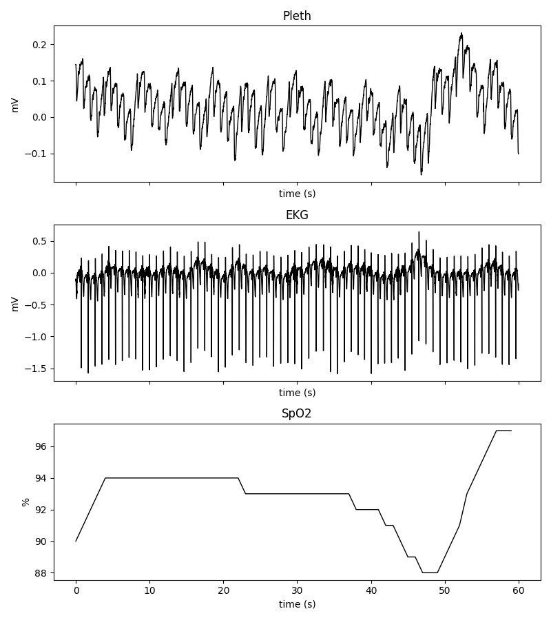
Visualizing raw signals
After loading the data, plot the raw signals:
from pyPSG.IO.plot import plot_raw_data

plot_raw_data(signals)
SpO2 signal processing
If a SpO2 channel is available, the signal is processed to extract oxygen saturation biomarkers.
First, retrieve the SpO2 signal and its sampling frequency:
spo2_signal = signals[channels["spo2"]]["signal"]
fs = signals[channels["spo2"]]["fs"]
Remove physiologically implausible values (below 50% or above 100%):
from pobm.prep import set_range

spo2_signal = set_range(spo2_signal)
Apply a median filter to smooth the signal:
from pobm.prep import median_spo2

spo2_signal = median_spo2(spo2_signal, FilterLength=301)
Create a corresponding time axis:
import numpy as np

time_signal = np.arange(0, len(spo2_signal)) / fs
Finally, compute SpO2 biomarkers:
from pyPSG.biomarkers.get_spo2_bm import extract_biomarkers_per_signal

spo2_bm = extract_biomarkers_per_signal(
    signal=spo2_signal,
    patient="Patient 1",
    time_begin=time_signal[0],
    time_end=time_signal[-1]
)
The resulting biomarkers are stored for later use.
PPG signal processing
If a PPG channel is available, the signal is processed to extract morphological features and derive physiological biomarkers.
Prepare the signal
Wrap the raw signal and its metadata into a structured object:
from dotmap import DotMap

ppg_signal = DotMap()
ppg_signal.v = signals[channels["ppg"]]["signal"]
ppg_signal.fs = signals[channels["ppg"]]["fs"]
ppg_signal.start_sig = 0
ppg_signal.end_sig = len(ppg_signal.v)
ppg_signal.name = "custom_ppg"
Preprocessing
Apply bandpass filtering and smoothing to obtain different signal representations:
import pyPPG.preproc as PP

filtering = True
fL = 0.5
fH = 12
order = 4
sm_wins = {"ppg": 50, "vpg": 10, "apg": 10, "jpg": 10}

prep = PP.Preprocess(fL=fL, fH=fH, order=order, sm_wins=sm_wins)

ppg_signal.filtering = filtering
ppg_signal.fL = fL
ppg_signal.fH = fH
ppg_signal.order = order
ppg_signal.sm_wins = sm_wins

ppg_signal.ppg, ppg_signal.vpg, ppg_signal.apg, ppg_signal.jpg = prep.get_signals(s=ppg_signal)
This step generates the filtered PPG signal and its derivatives (VPG, APG, JPG), which are required for feature extraction.
Fiducial point detection
Detect characteristic points in the PPG waveform:
import pyPPG.fiducials as FP
from pyPPG import PPG, Fiducials

s = PPG(s=ppg_signal, check_ppg_len=True)

fpex = FP.FpCollection(s=s)
ppg_fiducials = fpex.get_fiducials(s=s)

fp = Fiducials(fp=ppg_fiducials)
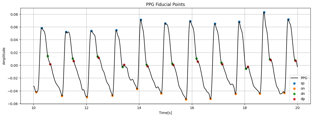
Fiducial points represent key landmarks in the waveform (e.g., systolic peak, dicrotic notch), which are essential for further analysis.
Visualize the detected fiducial points on the PPG waveform:
import matplotlib.pyplot as plt
import numpy as np

fid_df = fp.get_fp()

start = int(10 * s.fs)
end = int(20 * s.fs)

sig = s.ppg[start:end]
x = np.arange(start, end)

plt.figure(figsize=(15,5))
plt.plot(x, sig, color="black", label="PPG")

for col in ["sp", "on", "dn", "dp"]:
    idx = fid_df[col].dropna().astype(int)
    idx = idx[(idx >= start) & (idx < end)]

    plt.scatter(idx, s.ppg[idx], label=col)

plt.title("PPG Fiducial Points")
plt.xlabel("Samples")
plt.ylabel("Amplitude")
plt.legend()
plt.grid(True)

plt.show()
Biomarker extraction
Compute morphological biomarkers from the PPG signal:
import pyPPG.biomarkers as BM
from pyPPG import Biomarkers

bmex = BM.BmCollection(s=s, fp=fp)
bm_defs, bm_vals, bm_stats = bmex.get_biomarkers()

ppg_bm = Biomarkers(
    bm_defs=bm_defs,
    bm_vals=bm_vals,
    bm_stats=bm_stats
)
ECG signal processing
If an ECG channel is available, the signal is processed to detect cardiac events and extract clinically relevant biomarkers.
Preprocessing
Apply filtering to remove powerline interference and noise:
from pecg import Preprocessing as Pre
from pyPSG.utils import HiddenPrints

pre = Pre.Preprocessing(
    signals[channels["ecg"]]["signal"],
    signals[channels["ecg"]]["fs"]
)

# Remove powerline noise (50 Hz in Europe, 60 Hz in the US)
 with HiddenPrints(): # to avoid long verbose
    filtered_signal = pre.notch(n_freq=50)

# Apply bandpass filtering to remove baseline wander and high-frequency noise
filtered_signal = Pre.Preprocessing(
    filtered_signal,
    signals[channels["ecg"]]["fs"]
).bpfilt()
This step ensures that the ECG signal is clean and suitable for peak detection.
Fiducial point detection
Detect R-peaks and compute fiducial points:
from pecg.ecg import FiducialPoints as Fp

fp = Fp.FiducialPoints(
    filtered_signal,
    signals[channels["ecg"]]["fs"]
)

# Detect peaks using the jqrs algorithm
jqrs_peaks = fp.jqrs()

# Compute fiducial points using the Wavedet algorithm (MATLAB Runtime required)
matlab_path = "C:\Program Files\MATLAB\MATLAB Runtime\v910" # Replace this path with your local MATLAB Runtime installation path
ecg_fiducials = fp.wavedet(matlab_path, peaks=jqrs_peaks)
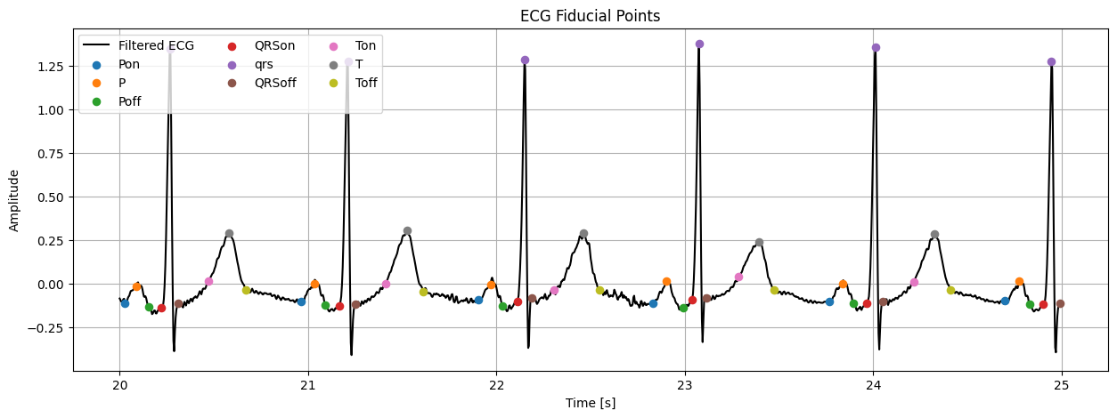
The Wavedet algorithm relies on MATLAB Runtime and is used to extract detailed ECG fiducial points.
Visualize the detected ECG fiducial points on the filtered ECG signal:
import matplotlib.pyplot as plt
import numpy as np

fs = signals["EKG"]["fs"]

start = int(20 * fs)
end = int(25 * fs)

sig = filtered_signal[start:end]
time = np.arange(start, end) / fs

fid = ecg_fiducials[0]

plt.figure(figsize=(15, 5))
plt.plot(time, sig, color="black", label="Filtered ECG")

fiducial_labels = [
    "Pon",
    "P",
    "Poff",
    "QRSon",
    "qrs",
    "QRSoff",
    "Ton",
    "T",
    "Toff"
]

for label in fiducial_labels:

    idx = fid[label]

    idx = idx[(idx >= start) & (idx < end)].astype(int)

    plt.scatter(idx / fs, filtered_signal[idx], zorder=5, s=35, label=label)

plt.xlabel("Time [s]")
plt.ylabel("Amplitude")
plt.title("ECG Fiducial Points")
plt.legend(ncol=3)
plt.grid(True)

plt.show()
Biomarker extraction
Compute interval- and waveform-based biomarkers:
from pecg.ecg import Biomarkers as Bm

bm = Bm.Biomarkers(
    filtered_signal,
    signals[channels["ecg"]]["fs"],
    ecg_fiducials
)

ints, stat_i = bm.intervals()
waves, stat_w = bm.waves()

ecg_bm = {
    "ints": ints,
    "stat_i": stat_i,
    "waves": waves,
    "stat_w": stat_w,
}
Heart rate variability (HRV) analysis
Heart rate variability (HRV) quantifies fluctuations in the time intervals between successive cardiac cycles.
In this analysis, HRV is derived from both ECG and PPG signals using peak-to-peak intervals.
ECG-based HRV
HRV computed from ECG signals is based on the intervals between successive heartbeats:
rr_intervals = np.diff(jqrs_peaks) / signals[channels["ecg"]]["fs"]
Compute HRV metrics:
from pyPSG.biomarkers import hrv_bms as hrv

hrv_bm = hrv.get_all_metrics(rr_intervals, 30)
PPG-based HRV
HRV can also be approximated from the PPG signal by analyzing the intervals between successive pulse peaks:
ppg_peaks = ppg_fiducials.sp
Compute the intervals between consecutive peaks:
rr_intervals = np.diff(ppg_peaks) / signals[channels["ppg"]]["fs"]
Compute HRV metrics:
ppg_hrv_bm = hrv.get_all_metrics(rr_intervals, 30)
This completes the multimodal analysis pipeline, demonstrating how physiological signals can be processed and transformed into meaningful biomarkers.